library(readxl)
library(reticulate)
library(tidyverse)
library(tidymodels)
library(tidytext)
library(text2vec)
library(embed)
library(umap)
library(uwot)
library(plotly)
library(GGally)
library(textstem)
library(SnowballC)
library(forcats)
library(tm)
library(dbscan)
library(factoextra)
library(cluster)
library(e1071)
library(quanteda)
library(here)

news_paper_data <- read_excel("C:/Users/LATITUDE 5520/Documents/Portfolio/Clustering_of_News_Articles/data/newspaper_data_raw.xlsx")


news_paper_data %>%
  head(n=2) %>%
DT::datatable(filter = "top")Introduction
The South African Institute of Civil Engineering (SAICE) published an Infrastructure Report Card (IRC) for South Africa in which the state of South Africa’s infrastructure is discussed. The report covers the following infrastructure: water, sanitation, solid waste management, roads, airports, airports, ports, oil and gas pipelines, rail, electricity, healthcare, fire, education and information and communication technology.
To accurately access South Africa’s infrastructure, SAICE requires data. However, data for each infrastructure category is not always available or incomplete. To improve the infrastructure evaluation accuracy, SAICE is interested in using data from online news articles. Towards this extent, SAICE has collected 9000 online articles in an Excel file.
Each row of the Excel file represents one news article and contains:
the article id,
the article title,
the article subtitle and
the article text.
Libraries and data loading
| Name | news_paper_data |
| Number of rows | 9000 |
| Number of columns | 5 |
| _______________________ | |
| Column type frequency: | |
| character | 2 |
| logical | 1 |
| numeric | 2 |
| ________________________ | |
| Group variables | None |
Variable type: character
| skim_variable | n_missing | complete_rate | min | max | empty | n_unique | whitespace |
|---|---|---|---|---|---|---|---|
| title | 2 | 1.00 | 3 | 143 | 0 | 8943 | 0 |
| article | 184 | 0.98 | 11 | 32971 | 0 | 8796 | 0 |
Variable type: logical
| skim_variable | n_missing | complete_rate | mean | count |
|---|---|---|---|---|
| subtitle | 9000 | 0 | NaN | : |
Variable type: numeric
| skim_variable | n_missing | complete_rate | mean | sd | p0 | p25 | p50 | p75 | p100 | hist |
|---|---|---|---|---|---|---|---|---|---|---|
| id | 0 | 1 | 13205.26 | 7650.51 | 2 | 5991.50 | 13408.5 | 20445.75 | 26134 | ▇▆▆▆▇ |
| …2 | 0 | 1 | 4500.50 | 2598.22 | 1 | 2250.75 | 4500.5 | 6750.25 | 9000 | ▇▇▇▇▇ |
We seem to have 5 variables instead of the 4 intended, we will remove the additional one.
We also see that the article variable contains 184 missing values, the title variable has 2 missing values while the subtitle section is empty everywhere.
We basically only have 2 variables of importance: article and title as the id is not informative.
Data Cleaning
The number of article with missing values is: 184 Text transformation
As we are dealing with text, we need to transform our data into a usable format by concatenating the rows of interests, removing any unwanted signs or numbers, extract tokens, and much more depending on the need.
corpus_df <- news_paper_df %>%
  unnest_tokens(word, article,
                token = "regex",
                pattern = "[^A-Za-z]+",
                to_lower = FALSE)

#Create the vocabulary of the articles
vocabulary <- corpus_df %>%
  select(word) %>%
  unique()

#Print the respective values
cat("The corpus contains", length(corpus_df$word),"tokens\n",
    "While the vocabulary has", length(vocabulary$word),"unique tokens")
The corpus contains 3340566 tokens
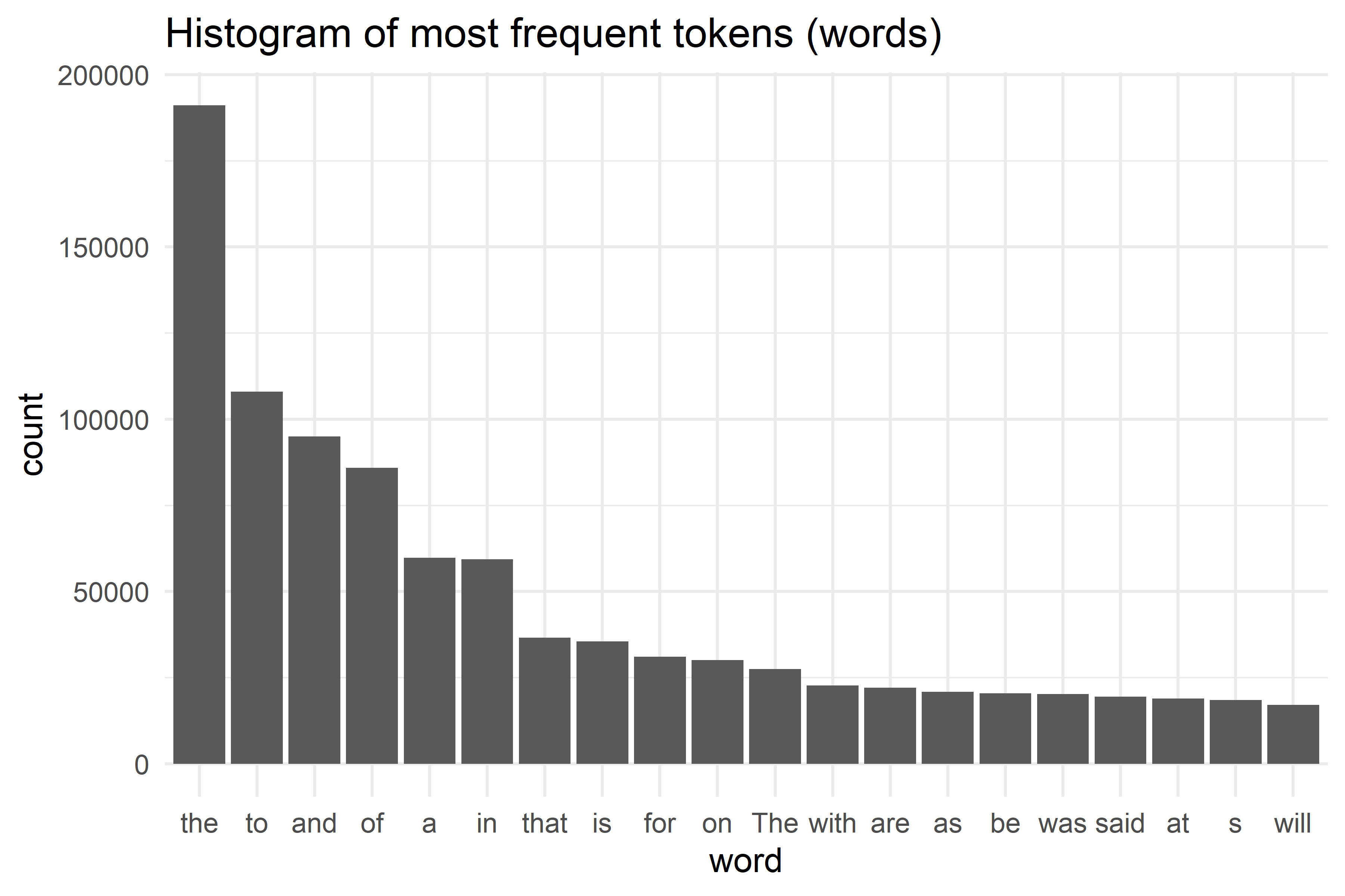
While the vocabulary has 76613 unique tokensLet us see the distribution of the most occurring words below:
top_20_tokens <- corpus_df %>%
  select(word) %>%
  count(word, name = "token_count") %>%
  arrange(desc(token_count)) %>%
  slice(1:20)

top_20_tokens %>%
  mutate(word = fct_reorder(word, -token_count)) %>%
  ggplot(aes(x = word, y = token_count)) +
  geom_bar(stat = "identity") +
  labs(
    title = "Histogram of most frequent tokens (words)",
    x = "word",
    y = "count"
  ) +
  theme_minimal()
Most of these are stop words (to, a, on, …) and also words are case-sensitive.
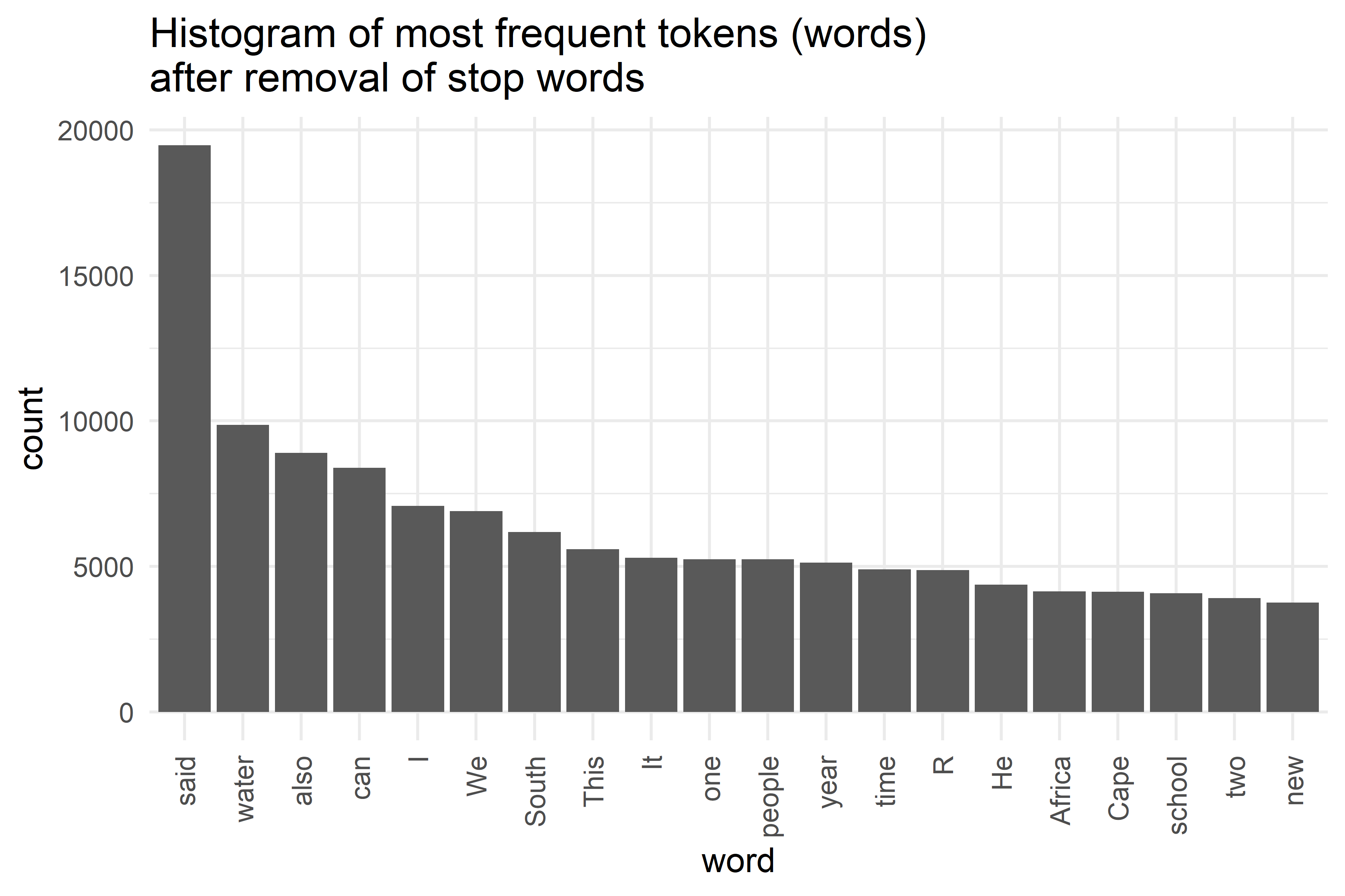
Let us compare now the most common words after removing the stop words:

Text normalisation
Let us perform some text normalisation by applying techniques such as case folding and stemming and see how that influences our vocabulary size:
The size of the vocabulary after case folding: 63770 The size of the vocabulary after stemming: 57246 The size of the vocabulary after case folding and stemming: 46696 Data quality transformation
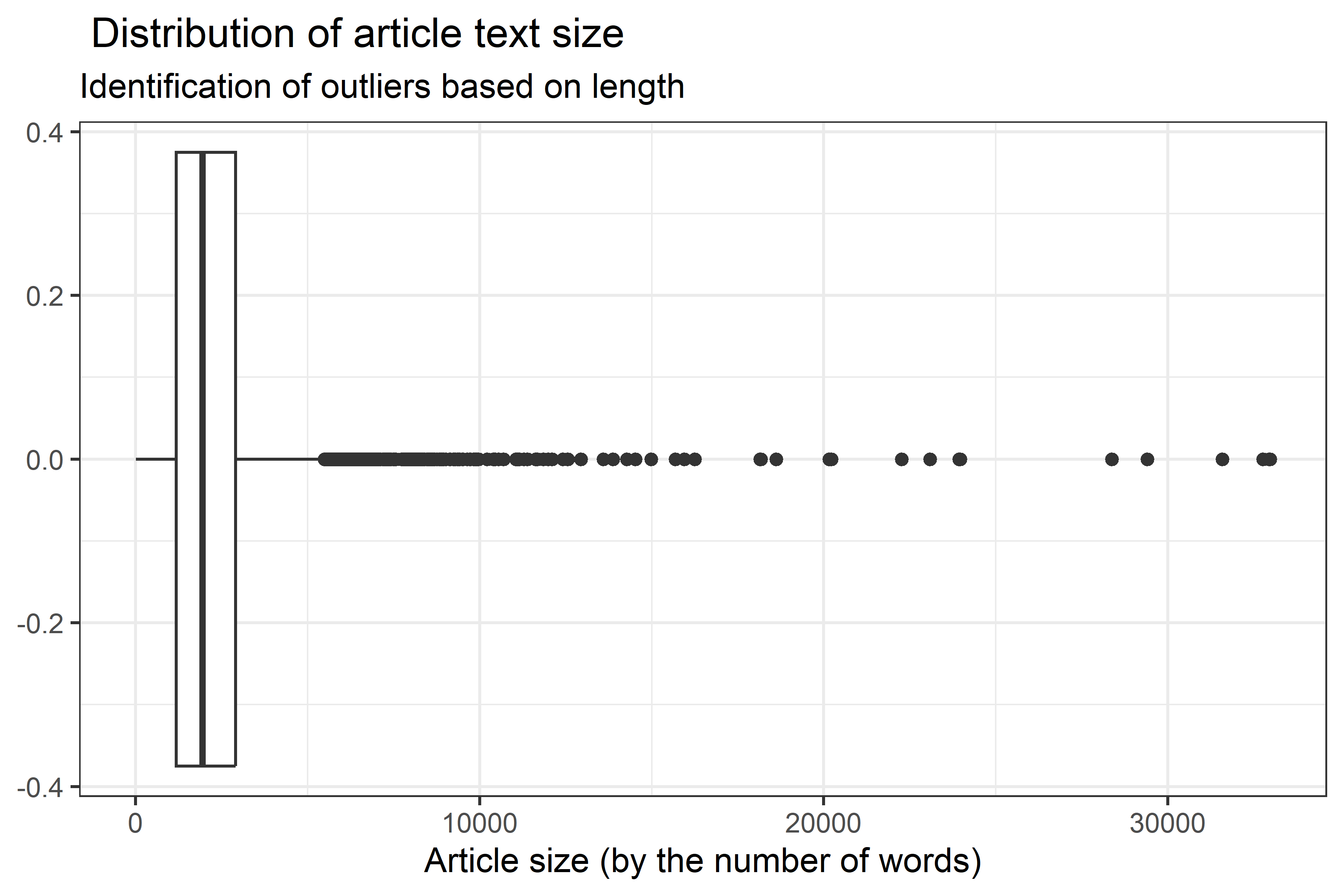
Could we have some articles that are way shorter than others?

The above plot showcases a strong distribution. For this reason, using a count vectorizer in modeling might not be the best option.
Instead, we should use a term frequency - inverse document frequency(tf-idf) vectoriser.
Let us remove articles that have less than 100 words:
news_paper_df %>%
  filter(article_length < 100) %>%
  count(name = "less than 100 words") %>%
  DT::datatable()
news_paper_df <- news_paper_df %>%
filter(article_length >= 100) Text embedding
As most algorithms cannot work with text directly, we will be transforming them using the following:
lemmatization;
stop words removal;
removing word having less than 2 letters;
number removal;
tf_idf;
removal of words appearing in less than 5 articles, which is different than words appearing only 5 times.
removing words that appear less than 5 times in the corpus
embedding <-
  news_paper_df %>%
  unnest_tokens(word, article,
                token = "regex",
                pattern = "[^A-Za-z]+") %>%
  filter(nchar(word) >= 2) %>%
  anti_join(get_stopwords()) %>%
  add_count(word, sort = TRUE) %>%
  group_by(word) %>%
  filter(sum(n) >= 5) %>%
  ungroup() %>%
  filter(n >= 5) %>%
  select(-n) %>%
  mutate(word = lemmatize_words(word)) %>%
  count(id, word, sort = TRUE) %>%
  bind_tf_idf(word, id, n)


## Let us extract the column names:
vocab <-
  embedding %>%
  select(word) %>%
  distinct() %>%
  pull(word)


## Embedding tibble
embedding_tbl <- embedding %>%
  select(-c(tf, idf, n)) %>%
  pivot_wider(names_from = word, values_from = tf_idf,
              values_fill = 0, names_repair = "unique") %>%
  rename(id = id...1)


embedding_tbl
Each row here represents a single article and each column a unique token (word).
Let us analyse the tf-idf of the 873th document for example and see what it is about:
First we look at the article’s content below:
[1] "The NDK0 11kV Oil Circuit Breaker at the Nivensdrift substation tripped, affecting Nivensdrift, Kruisrivier, and the surrounding areas. Staff attending to restoration of supply, no timeframe available. We apologise for the inconvenience caused."The article appears to be electricity.
Below is the repartition of the top 10 word with the highest tf-idf:
# A tibble: 10 × 4
      id word              n tf_idf
   <dbl> <chr>         <int>  <dbl>
 1  4038 breaker           1  0.321
 2  4038 timeframe         1  0.312
 3  4038 kv                1  0.307
 4  4038 restoration       1  0.264
 5  4038 circuit           1  0.250
 6  4038 oil               1  0.221
 7  4038 apologise         1  0.219
 8  4038 substation        1  0.215
 9  4038 inconvenience     1  0.210
10  4038 trip              1  0.187
Which document is most similar to the 873th document according to the tf-idf embeddings?
# A tibble: 5 × 2
     id similarity[,1]
  <dbl>          <dbl>
1  4038          1
2  3992          0.645
3  4047          0.574
4  1270          0.335
5 18491          0.239
Below are the top 10 words of the article (id=3992) which is the most similar to the 873th article based on cosine similarity:
# A tibble: 10 × 4
      id word              n tf_idf
   <dbl> <chr>         <int>  <dbl>
 1  3992 timeframe         1  0.330
 2  3992 restoration       1  0.279
 3  3992 apologise         1  0.231
 4  3992 inconvenience     1  0.223
 5  3992 outage            1  0.196
 6  3992 surround          1  0.190
 7  3992 section           1  0.175
 8  3992 party             1  0.161
 9  3992 deal              1  0.149
10  3992 attend            1  0.148
Dimensionality reduction
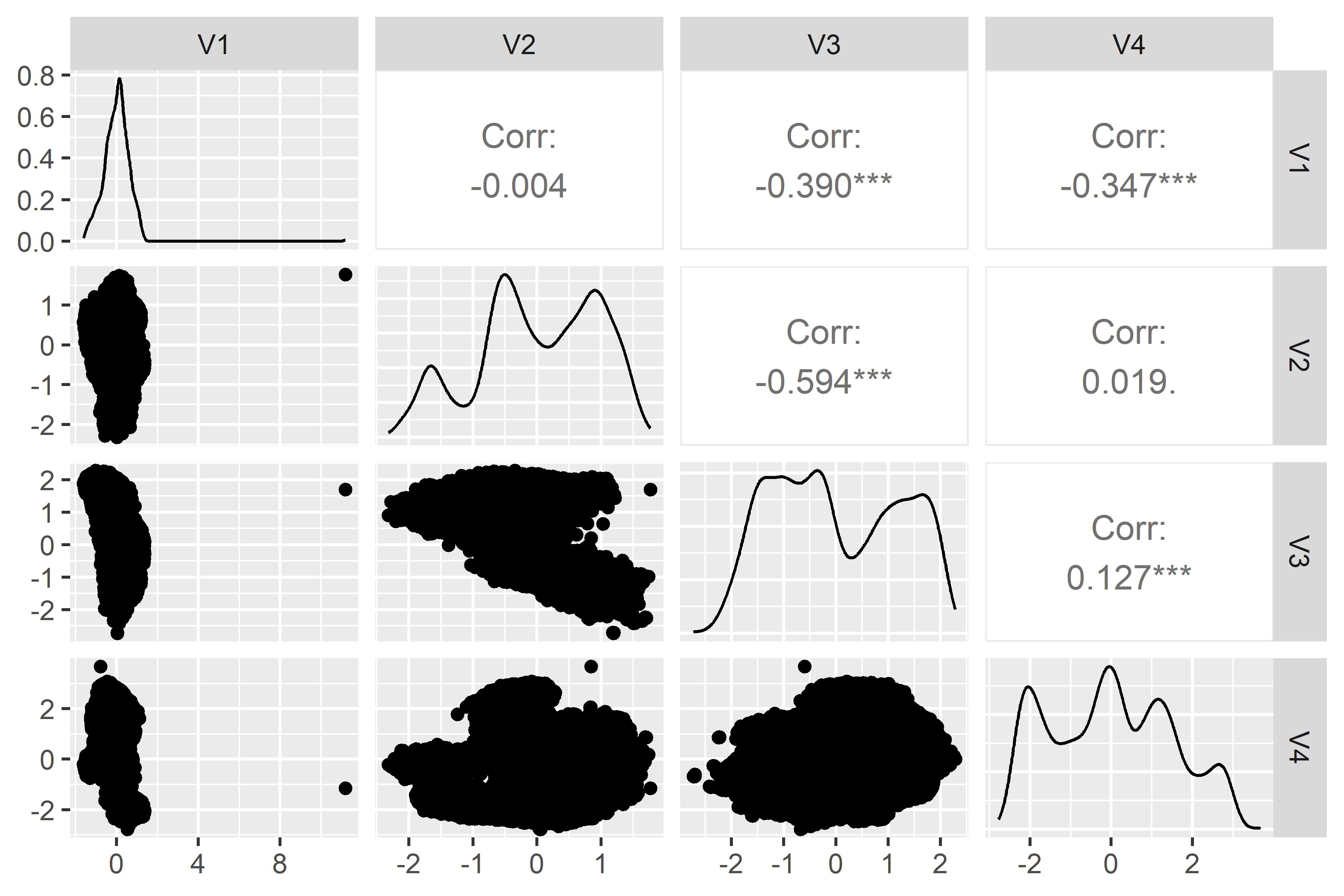
Most clustering algorithms become slow in the presence of high dimensional data. To alleviate this, we perform dimensionality reduction using the UMAP algorithm and we reduce it to only 4 components:
umap <- uwot::umap(embedding_tbl[,-1], n_components = 4, seed = 2024)# A tibble: 8,793 × 4
V1 V2 V3 V4
<dbl> <dbl> <dbl> <dbl>
1 -0.0964 1.09 -1.36 -1.33
2 -0.562 0.968 -1.38 -0.165
3 -0.145 0.705 -0.632 -0.190
4 -0.171 1.10 -0.816 0.0783
5 -0.0239 0.178 0.0301 -0.258
6 0.0837 1.11 -0.912 -0.285
7 0.379 1.47 -1.55 -0.841
8 -0.271 1.33 -0.483 0.0136
9 -0.157 1.28 -1.17 -0.504
10 -0.432 1.21 -1.29 -0.240
# ℹ 8,783 more rows
Voilà!
We notice that we have a big cluster and some little cluster(s) as well which could indicate a group of articles that are similar to one another and dissimilar to most of the articles. These small clusters could also be outliers.
Also besides umap, we could try other clustering algorithms such as SOM or even DBSCAN and see whether clusters are more visible than this.
As for now, thank you for your attention and see you soon. 🖖